This article is coauthored by A2L Consulting’s CEO, Kenneth J. Lopez, J.D., a trial graphics and trial consulting expert and David H. Schwartz, Ph.D. of Innovative Science Solutions. Dr. Schwartz has extensive experience designing programs that critically review the scientific foundation for product development and major mass tort litigation. For 20 years, he has worked with the legal community evaluating product safety and defending products such as welding rods, cellular telephones, breast implants, wound care products, dietary supplements, general healthcare products, chemical exposures (e.g., hydraulic fracturing components), and a host of pharmaceutical agents (including antidepressants, dermatologics, anti-malarials, anxiolytics, antipsychotics, and diet drugs).

[See also follow-up article discussing the null hypothesis] 

Many of us have been there in the course of a trial or hearing. An expert or opposing counsel starts spouting obscure statistical jargon. Terms like "variance," "correlation," "statistical significance," "probability" or the "null hypothesis." For most, especially jurors, such talk can cause a mental shutdown as the information seems obscure and unfamiliar.

It’s no surprise that talk of statistics causes confusion in a courtroom setting. Sometimes, a number can be much higher than another number and yet the finding will not be statistically significant. In other instances, a number can be nearly the same as its comparison value and this difference can be highly statistically significant.

Helping judge and jury develop a clear and accurate understanding of statistical principles is critical – and using the right type of trial graphics can be invaluable. 

Let’s demonstrate this by way of example.

Suppose we want to know whether a petroleum refinery increases the level of benzene in fish that inhabit the coastal waters near the refinery.

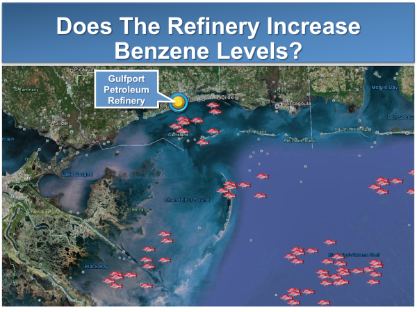
The hypothesis is that the benzene level in the coastal fish near the refinery (the Refinery Fish) is higher than the benzene level in off-shore fish that live in waters far from the refinery (the Control Fish).

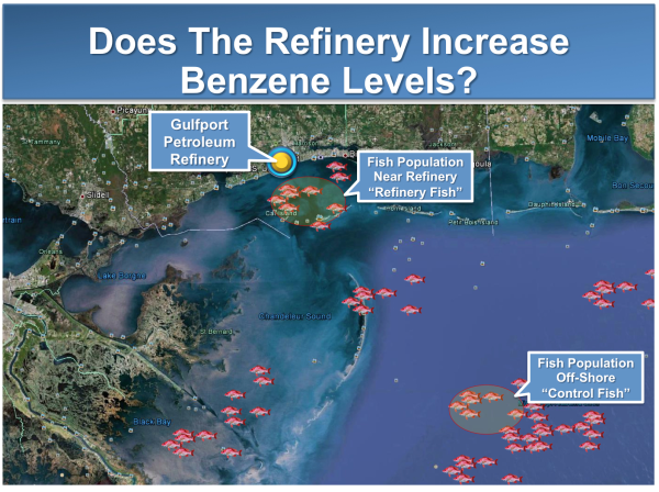
Because we can never collect every single fish and measure benzene levels in all of them, we will never know the precise answer to the hypothesis (not to mention the fact that if we did, the study would be irrelevant because there would be no more fish). But we can sample some of the fish near the refinery and then compare the benzene levels in these fish to a sample of fish collected from the middle of the sea. Statistical techniques are a clever tool that we use to answer the research question, even though we haven't measured all the fish in each location.

Unless one is trained in statistics, the evaluating might appear easy and straightforward. Simply compare benzene levels in the Refinery Fish sample to the benzene levels in the Control Fish sample and see which is higher. But what if our sample only reveals a very small difference between the benzene levels in the Refinery Fish sample compared to the Control Fish sample? How do we know if that difference we observed in our samples is a real difference (i.e., potentially due to a causal relationship with the refinery) or whether it was simply due to our sampling techniques (i.e., due to chance)? Statistical techniques provide us with a way to properly interpret our findings.

An overview of well-established statistical techniques surrounding hypothesis testing is in the trial graphic below:

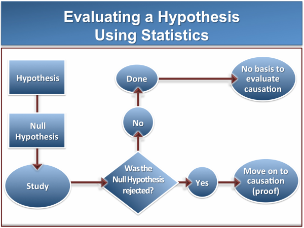
While this graphic is somewhat oversimplified, it does provide the basic steps that are taken in the hypothesis testing decision tree.

Although imperfect [pdf], a criminal case serves as a useful analogy to help understand how statistics work. In a criminal case, the defendant is assumed to be innocent unless proven guilty beyond a reasonable doubt. In statistical terms, the overall trial can be likened to statistical testing of a hypothesis (i.e. did he do it?), and the presumption of innocence can be likened to the "null hypothesis." Like the null hypothesis, the starting point in a criminal trial is that defendant is not guilty, and in statistical terms, that the connection you've set out to establish is just not there. The trial graphics below provide an overview of this concept. Again, this is an imperfect metaphor and is subject to criticism from a pure statistical vantage point. Neverteless, it provides some assistance to the novice in clarifying the fundamental tenets of hypothesis testing.

Returning to our refinery hypothetical, we form our null hypothesis.

In this case, the null hypothesis is that the Refinery Fish are exactly the same as all the other fish in the ocean in terms of benzene levels — specifically, that they come from the same population. Succinctly, the null hypothesis is as follows:

In our study, as in all scientific studies, we will be testing how likely it is that we would obtain dataat least as extreme as our data if the null hypothesis were true. In other words, we will be evaluating the conditional probability of obtaining the data that we observe.

In plain English, proper statistical testing means assuming your hypothesis is wrong and then evaluating the likelihood that you would come up with the findings that you did. Statistical testing is not about proving things true. Rather, it is about proving that the alternative — i.e. your null hypotheses — is likely not true. Only then can we reject the null hypothesis and conclude that our research hypothesis is plausible.

Determining whether or not it is reasonable to reject the null hypothesis is done by collecting data in a scientific study. Here, we start by measuring benzene levels in two samples of fish: (1) a group of fish near the refinery (Refinery Fish); and . . . 

(2) a group of fish in the middle of the ocean, nowhere near the refinery (Control Fish).

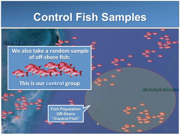
We will then calculate an average benzene level in each group of fish, which will serve as a reasonable estimate of the benzene level in each population of fish (i.e., all fish living near the refinery and all fish not living near the refinery). Of course, how we take our samples is a critical component of the study design, but we will assume for this example that we have used appropriate sampling techniques.

Let's examine 3 possible outcomes in the trial graphics below. The first possibility will deal with an obvious result.

In this example, let's assume that every fish in the Refinery Fish sample had a benzene level of 10, and every fish in the Control Fish sample had a benzene level of 1. Thus, the average Refinery Fish benzene level is 10 and the average Control Fish benzene level is 1. When we do our statistical test, we calculate the conditional probability – i.e., the probability that we would have obtained this dramatic difference (10 vs. 1) given that the null hypothesis is true. This probability is called a "p value."

In this case, the p value is so low (let's say: p = 0.00000001) that we reject the null hypothesis. Stated another way: The probability of obtaining such extreme data if the null hypothesis were true is 0.0000001. Based on this analysis, it doesn’t make sense to believe that we would have obtained these results if the null hypothesis were true. So we reject the null hypothesis.

Our study was a success. We reject the null hypothesis, and we draw a clear-cut conclusion -- i.e., the Refinery Fish come from a different population of fish with respect to benzene levels. So we conclude that the refinery, absent other factors, may have something to do with the benzene levels in these fish. Because this difference was so clear-cut (every single fish in the Refinery Fish sample had extremely high benzene levels and every single fish in the Control Fish sample had extremely low values), we didn’t even need statistics to get our answer.

Now let's look at another, more realistic, possibility. This time the difference between the two samples is a little less clear cut.

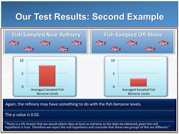
In this example, the average benzene level in the Refinery Fish sample is 8 and the average benzene level in the Control Fish sample is 3. When we do our statistical test, we learn that the p value is 0.02. Said another way, the probability that we would have obtained these findings, given that the null hypothesis is true, is about 2%.

Thus, as with the extreme example above, the probability of obtaining these findings, given that the null hypothesis is true is very low (not quite as low as in the prior example, but still pretty low). This raises the question: how low a probability is low enough?

Traditionally, statisticians have used a “cut-off” probability level of 5%. If the probability of obtaining a certain set of results is less than 5% (given the null hypothesis), then scientists and statisticians have agreed that it is reasonable to reject the null hypothesis. In this case, we reject the null hypothesis and conclude that the Refinery Fish must come from a different population than the Control Fish. Again, as with the earlier example, we conclude that the refinery must have something to do, absent other factors, with the benzene levels.

So far, so good. Now, let's do one more. This time let's assume that the difference between the Refinery Fish sample and the Control Fish sample has gotten much smaller.

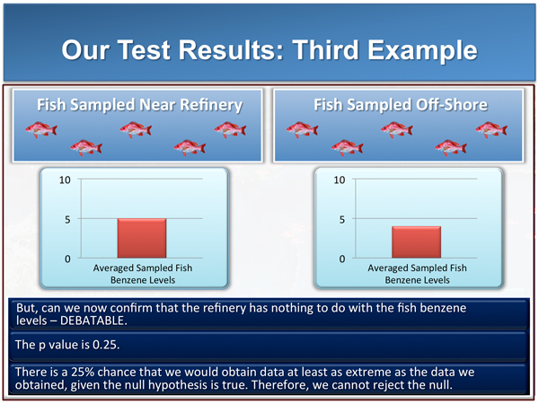
In this example, the average benzene level in the Refinery Fish sample is 5 and the average benzene level in the Control fish sample is 4. The benzene levels, on average, are numerically higher in the Refinery Fish compared to the Control Fish. But are they statistically higher? In statistical terms, how likely would it be to obtain these findings if all the fish were the same with respect to their benzene levels? In other words, is it reasonable to conclude we would have obtained findings this extreme if the refinery had nothing to do with the benzene levels?

When we do our statistical test, we learn that the p value is 0.25. Thus, the probability that we would have obtained findings this extreme, given that the null hypothesis is true, is about 25%. One in four times that we take these samples, we will get findings like this if the null hypothesis is true.

A twenty-five percent chance is not so unlikely. It certainly doesn't meet the 5% cut-off rule (i.e., less than 5%). Therefore, statistical best practices tell us that we cannot reject the null hypothesis.

But what does it mean when we cannot reject the null hypothesis? Can we conclude that the null is true? This is actually a critical question, and it represents an area where statistics often get misused in court, in trial graphics, in the media and elsewhere. And what about other intervening factors like bias and confounding?

Our next posts on using trial graphics and statistics to win or defend your case will grapple with these important questions. Please do leave a comment below (your email address is not displayed or shared).

[See also follow-up article discussing the null hypothesis] 

Other A2L Resources related to this article:

• Teaching science to a jury using trial graphics
• Trial graphics consultants at A2L Consulting
• Conveying size or scale to judges and juries with trial graphics
• Free Download: The Energy/Environmental Litigation Trial Graphics Toolkit
• Using scale models as trial graphics and demonstrative evidence
• Simplifying complex cases with trial graphics
• Contact an A2L Consulting office
• DOWNLOAD - The BIG Litigation Interactive E-Book